Skin Space: Modeling Skin Color in Images

Introduction

Skin color is a common method for detection/recognition of humans in low level computer vision methods. In particular it is typical to use this cue for hand and face detection, especially in applications where a camera is the only available data source (i.e., no IR camera like is used in the Xbox Kinect). Although skin color can be a useful cue it is quite noisy - susceptible to any changes in lighting. Equally as problematic is the fact that skin color, while fairly distinct as compared to coloring among natural images, is highly non- seperable from the rest of the color distribution of natural images.

This is just a little exploration of skin color modeling using the Pratheepan dataset. It’s not a comprehensive review and doesn’t reveal anything earth- shaterring but is more of a demonstration of data exploration using pandas, IPython, and matplotlib as well as a look at the strengths and weaknesses of skin segmentation as a human detection method.

HUGE thanks to Mr. Mohd Zamri for preparing the Pratheepan dataset that we use in this exercise. You can download the original dataset here. I used the dataset to create an sqlite database as seen below. If you’re interested in getting the sqlite version of the dataset please contact me and I’ll find a way to get it to you.

Cracking open the Pratheepan dataset

In [1]:

# do all the typical importing first
%matplotlib inline
import matplotlib.pyplot as plt
import pandas as pd
import sqlite3
import numpy as np
plt.style.use('ggplot') # set a new matplotlibrc for nicer looking plots

# This disables (the all-too-often falsely triggered) 'SettingWithCopyWarning'
pd.options.mode.chained_assignment = None # we promise we'll be careful

# open a connection to our sqlite file
conn = sqlite3.connect('prath.sqlite')
curs = conn.cursor()

print "pandas:",pd.version.short_version
print "numpy:",np.version.short_version

Out [1]:

pandas: 0.16.2
numpy: 1.8.2

Load per-pixel data from the pixels table.

In [2]:

q = "select image_id,pixel_index,skin,r,g,b from pixels order by image_id,pixel_index"
prath = pd.read_sql_query(q,conn)

# index the dataframe by image_id and pixel_index for easier access and conversion to images
prath.set_index(['image_id','pixel_index'],inplace=True)
prath.head()

Out [2]:

		skin	r	g	b
image_id	pixel_index
0	0	0	210	205	202
	1	0	211	206	203
	2	0	213	208	205
	3	0	216	211	208
	4	0	219	214	211

The images table contains all the image metadata.

In [3]:

images = pd.read_sql("select * from images",conn,index_col='file_name')
images.head()

Out [3]:

	image_id	width	height
file_name
sri-lankan-actress-Natasha-Perera-	0	286	400
Megan-Fox-Pretty-Face-1-1024x768	1	512	384
Kishani_-__n_-_5	2	239	320
yamuna_erandathi	3	276	400
pg42RF	4	300	362

Let’s take a quick sample of the images in the dataset for demonstration. Notice the skin colors and lighting conditions are pretty diverse among the sample.

In [4]:

fig, axes = plt.subplots(4,4,subplot_kw=dict(xticks=[],yticks=[]))
imageIDs = pd.read_sql_query("select image_id from images",conn).values
sample_images = np.random.choice(imageIDs.ravel(),16,replace=False)

for img_id,ax in zip(sample_images,axes.ravel()):
    w,h = list(*curs.execute("select width,height from images where image_id=%d" % img_id))
    df = prath.loc[(img_id,),'r':'b'].astype(np.uint8)
    
    ax.imshow(df.values.reshape(h,w,3))
    
fig.tight_layout()
fig.set_size_inches(fig.get_size_inches()[0]*1.5, fig.get_size_inches()[1]*1.5)
fig.subplots_adjust(wspace=0,hspace=0)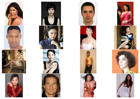

Out [4]:

A baseline model - Logistic Regression on the RGB space

Just as a starting point, let’s see how well we can do with one of the simplest of classification models - Logistic Regression or logit regression - just using the first and second order RGB pixels. The second degree RGB features will allow us to get a curved decision boundary from the logit model which gives us a little more flexibility.

In [5]:

from StringIO import StringIO
def report(y,predy):
    '''A simple report generator for evaluating model accuracy'''
    ret = StringIO()
    acc = np.sum(y == predy)
    fn = np.sum((y != predy) & (y == True))
    fp = np.sum((y != predy) & (y == False))
    dispstr = lambda l,m: "%s: %d/%d (%.3f%%)" % (l,m,y.shape[0],100.0*m/y.shape[0])
    print >> ret, dispstr("Accuracy", acc)
    print >> ret, dispstr("FN", fn)
    print >> ret, dispstr("FP", fp)
    return ret.getvalue()

In [6]:

from sklearn.linear_model import LogisticRegression
from sklearn.cross_validation import train_test_split

clf_rgb = LogisticRegression(C=1e-3)
prath['r2'] = prath['r']**2
prath['g2'] = prath['g']**2
prath['b2'] = prath['b']**2
train, test = train_test_split(prath,train_size=0.5)

get_rgb_features = lambda df: df.loc[:,'r':'b2']

print clf_rgb.fit(get_rgb_features(train),train['skin'])
print report(test.skin, clf_rgb.predict(get_rgb_features(test)))

Out [6]:

LogisticRegression(C=0.001, class_weight=None, dual=False, fit_intercept=True,
          intercept_scaling=1, max_iter=100, multi_class='ovr',
          penalty='l2', random_state=None, solver='liblinear', tol=0.0001,
          verbose=0)
Accuracy: 2195411/2956654 (74.253%)
FN: 526170/2956654 (17.796%)
FP: 235073/2956654 (7.951%)

About 74% accuracy on our test dataset overall - not bad. But let’s take a random image to get another view on how the model is performing.

In [7]:

def plot_thresh(img,predimg,mask):
    '''Display the results of applying a skin pixel classifier to an image'''
    fig, (ax1,ax2,ax3,ax4) = plt.subplots(1,4,subplot_kw=dict(xticks=[],yticks=[]))
    
    ax1.imshow(img)
    ax2.imshow(predimg,interpolation='nearest',cmap='gray')
    ax2.set_title('backprojection')
    threshimg = np.zeros_like(img)
    threshimg[predimg >= 0.5] = 255
    ax3.imshow(threshimg)
    ax3.set_title('threshold')
    ax4.imshow(mask,interpolation='nearest',cmap='gray')
    ax4.set_title('ground truth')

In [8]:

def get_image(fn):
    '''Helper function to get an rgb image from its name'''
    if isinstance(fn,basestring):
        img_id,w,h = images.loc[fn]
    else:
        img_id,w,h = images[images.image_id==fn].iloc[0]
    df = prath.loc[(img_id,),:]
    
    # the .values property is not totally dependable. But it works in this instance
    blocks = df.loc[:,'r':'b']
    img = blocks.values.astype(np.uint8).reshape(h,w,3)
    
    return df,img

In [9]:

buffydf, buffy = get_image('06Apr03Face')
buffydf['r2'] = buffydf['r']**2
buffydf['g2'] = buffydf['g']**2
buffydf['b2'] = buffydf['b']**2

pred = clf_rgb.predict_proba(get_rgb_features(buffydf))[:,1] # select only the skin=True probability
predimg = pred.reshape(buffy.shape[:2])
mask = buffydf['skin'] == 1

plot_thresh(buffy,predimg,mask.reshape(buffy.shape[:2]))

plt.gcf().tight_layout()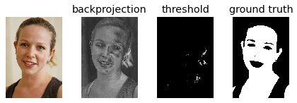

Out [9]:

In this case, the skin segmentation result is practically useless. This is a demonstration of the high false negative rate (FNR) we saw in the model evaluation. It also shows the model is falsely classifying light colored hair as skin but this seems like less of a problem since the color is perceptually close to skin color.

Exploring skin pixels in the YCrCb colorspace

One of the things we haven’t discussed yet is how lighting environment effects the results of our classifier. Ideally, we would want a skin color classifier to be insensitive to changes in lighting in order to be useful in any practical setting. One of the ways we can mitigate lighting effects is by using a color space that approximately separates intensity or luminosity from the chromaticity. There are several such possible models including HSV (Hue- Saturation-Value), LUV (Luminosity-UV), and others. Here I’ve decided to use the YCrCb encoding of the RGB space.

YCrCb (or YCC) was originally created for the transmission of digital video because of its flexibility in badwidth usage. Since humans are much more sensitive to illumination than they are to color, the CrCb components of the signal can be downsampled significantly with little impact on the perceived image quality. This encoding is also practical since it is a simple linear mapping from the RGB space.

In the figure below, you can see the roughly elliptical distribution of skin pixels in the CrCb space. The plot on the right also gives some idea of how much these values overlap with non-skin pixels in the Pratheepan dataset.

In [10]:

def add_crcb(df):
    # grabbed from http://www.equasys.de/colorconversion.html
    df['Y'] =   0.299  *df['r'] + 0.587  *df['g'] + 0.114  *df['b']
    df['Cr'] =  0.5    *df['r'] - 0.419  *df['g'] - 0.081  *df['b'] + 128
    df['Cb'] = -0.169  *df['r'] - 0.331  *df['g'] + 0.5    *df['b'] + 128
add_crcb(prath)

In [11]:

def plot_density(df=None,colorbar=True,H=None,**kwargs):
    if H is None:
        H, xedges, yedges = np.histogram2d(df['Cr'].values, df['Cb'].values,bins=np.arange(0,257))
    else:
        xedges = yedges = np.arange(257)

    # flip the histogram axes so plot displays CrCb values propery
    Hp = H.T
    
    ax = plt.gca()
    fig= plt.gcf()
    mesh = ax.pcolormesh(xedges,yedges,np.ma.masked_where(Hp == 0,Hp,copy=False),**kwargs)

    if colorbar: cbar = fig.colorbar(mesh)
    ax.set_xlabel('Cr')
    ax.set_ylabel('Cb')
    ax.set_xlim(115,205)
    ax.set_ylim(70,145);
    ax.grid()
    
    return H

In [12]:

fig, (ax1,ax2) = plt.subplots(1,2)

plt.sca(ax1)
ax1.set_title('CrCb Skin pixel distribution')

# be nice to numpy and give it a singly indexed dataframe
Hs = plot_density(prath[prath.skin==1])

# note: we add 1 extra bin to the histogram to avoid binning together values of 254 and 255 
#(see notes on numpy doc http://docs.scipy.org/doc/numpy/reference/generated/numpy.histogram.html)
Hns, xedges, yedges = np.histogram2d(prath[prath.skin==0]['Cr'].values, prath[prath.skin==0]['Cb'].values,bins=np.arange(257))
Hdiff = Hs-Hns

plt.sca(ax2)
ax2.set_title('Skin pixels - Non-skin pixels')
plot_density(H=np.ma.masked_where(Hdiff < 0, Hs, copy=True))

fig.set_size_inches(fig.get_size_inches()[0]*2, fig.get_size_inches()[1])
fig.tight_layout()

print "Uniquely seperable skin/non-skin pixels: \n\t%.2f %%" % (100*(np.sum(Hs[Hns==0]) + np.sum(Hns[Hs==0]))/len(prath))

# Create a dataframe with the counts for each CrCb value
crcbspace = np.mgrid[:256,:256].T.reshape(-1,2)
counts = pd.DataFrame(np.hstack((crcbspace,Hdiff.T.reshape(-1,1))),columns=['Cr','Cb','n'])
merged = prath.merge(counts,on=['Cr','Cb'],how='outer')

print "Majority Thresholding classifier"
print "\t"+"\n\t".join(report(merged.skin,merged.n >= 0).split("\n"))

Out [12]:

Uniquely seperable skin/non-skin pixels: 
	10.61 %
Majority Thresholding classifier
	Accuracy: 4361413/5978842 (72.947%)
	FN: 1551894/5978842 (25.956%)
	FP: 0/5978842 (0.000%)

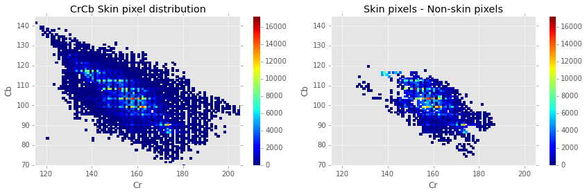
The plot above empirically shows that only a small minority (~10.6%) of pixels in the CrCb pixels can be uniquely separated into skin and non-skin pixels. It’s also shown that if we were to build a rudimentary classifier, assigning category based on a majority vote of skin and non-skin pixels for that value, we could achieve a classification accuracy of about 73%.

Let’s try fitting a logit model to the CrCb skin pixels

Now we’ll compare how a logit model performs on the CrCb space.

In [13]:

prath['Cr2'] = prath['Cr']**2
prath['Cb2'] = prath['Cb']**2
prath['CrCb'] = prath['Cr']*prath['Cb']

clf_crcb = LogisticRegression(C=1)
train, test = train_test_split(prath,train_size=0.5)

get_ycc_features = lambda df: df.loc[:,'Cr':'CrCb']

print clf_crcb.fit(get_ycc_features(train),train.skin)
print report(test.skin, clf_crcb.predict(get_ycc_features(test)))

Out [13]:

LogisticRegression(C=1, class_weight=None, dual=False, fit_intercept=True,
          intercept_scaling=1, max_iter=100, multi_class='ovr',
          penalty='l2', random_state=None, solver='liblinear', tol=0.0001,
          verbose=0)
Accuracy: 2376578/2956654 (80.381%)
FN: 310298/2956654 (10.495%)
FP: 269778/2956654 (9.124%)

Again, we’ll take a look at the sample image we used before.

In [14]:

add_crcb(buffydf)
buffydf['Cr2'] = buffydf['Cr']**2
buffydf['Cb2'] = buffydf['Cb']**2
buffydf['CrCb'] = buffydf['Cr']*buffydf['Cb']

In [15]:

pred = clf_crcb.predict_proba(get_ycc_features(buffydf))[:,1] # select only the skin=True probability
predimg = pred.reshape(buffy.shape[:2])

plot_thresh(buffy,predimg,(buffydf['skin'] == 1).reshape(buffy.shape[:2]))
plt.gcf().tight_layout()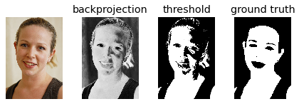

Out [15]:

At least on this sample image, our CrCb logit model is performing much better. The model is still picking up small sections of hair but nothing too troubling. It’s also apparent here how the uneven lighting is affecting the results of the classifier.

A hard threshold model for comparison

Just as an additional model to compare against, we create a classifier that uses a hard threshold on CrCb values chosen by hand.

In [16]:

hard_thresh = [(150,180),(85,115)]
def skinthresh(ds,thresh):
    (cr_lo,cr_hi),(cb_lo,cb_hi) = thresh
    return (cr_lo <= ds['Cr']) & (ds['Cr'] <= cr_hi) & (cb_lo <= ds['Cb']) & (cb_hi <= ds['Cb'])
pred = skinthresh(test,hard_thresh)
print report(test.skin, pred)

Out [16]:

Accuracy: 2140751/2956654 (72.405%)
FN: 769284/2956654 (26.019%)
FP: 46619/2956654 (1.577%)

In [17]:

predimg = skinthresh(buffydf,hard_thresh).reshape(buffy.shape[:2])
plot_thresh(buffy,predimg,(buffydf['skin'] == 1).reshape(buffy.shape[:2]))
plt.gcf().tight_layout()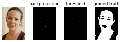

Out [17]:

Logit Decision Boundary

To get a better idea of our Logit fit, we’ll take a look at its decision boundary.

In [18]:

def decision_bound(clf,X,y,n=1000):
    theta = np.array(list(clf.intercept_) + list(clf.coef_.ravel()))
    subset = np.random.choice(X.index.values,n,replace=False)
    
    X,y = X.ix[subset], y.ix[subset]
    mask = y == 1

    plt.plot(X['Cr'][mask],X['Cb'][mask],'o',label='Skin',alpha=0.8)
    plt.plot(X['Cr'][~mask],X['Cb'][~mask],'o',label='NonSkin',alpha=0.1)

    plt.gca().set_xlabel('Cr')
    plt.gca().set_ylabel('Cb')
    plt.gca().set_xlim(115,205)
    plt.gca().set_ylim(70,145)
    plt.grid(True)

In [19]:

fig,(ax1,ax2) = plt.subplots(1,2)

N = 1000 # sqrt of the number of points to use for the grid
theta = clf_crcb.coef_.ravel()

# evaluate the decision function over a (sparse) grid of points
cr = np.linspace(np.min(prath['Cr']),np.max(prath['Cr']),N).reshape(1,N)
cb = np.linspace(np.min(prath['Cb']),np.max(prath['Cb']),N).reshape(N,1)
z = theta[0]*cr + theta[1]*cb + theta[2]*cr**2 + theta[3]*cb**2 + theta[4]*cr*cb + clf_crcb.intercept_

plt.sca(ax1)
decision_bound(clf_crcb,train.loc[:,'Cr':'Cb'],train.skin,n=30000)
ax1.contour(cr.ravel(),cb.ravel(),z,[0],label='Logit',linewidths=2.5,alpha=0.7)

plt.sca(ax2)
plot_density(train[train.skin == 1],alpha=0.5,colorbar=False)
ax2.contour(cr.ravel(),cb.ravel(),z,[0],label='Logit',linewidths=2.5,alpha=0.7)

x1 = np.array(hard_thresh[0])
x2 = np.array(hard_thresh[1])
ax1.add_patch(plt.Rectangle([x1[0],x2[0]],x1[1]-x1[0],x2[1]-x2[0],fill=False,ls='dashed',lw=3,color='m',label='Threshold'))
ax2.add_patch(plt.Rectangle([x1[0],x2[0]],x1[1]-x1[0],x2[1]-x2[0],fill=False,ls='dashed',lw=3,color='m',label='Threshold'))

line_proxy = plt.Line2D([],[],color='b',ls='solid',lw=2.5)
handles, labels = ax1.get_legend_handles_labels()
ax1.legend(handles+[line_proxy],labels+['Logit'])

handles, labels = ax2.get_legend_handles_labels()
ax2.legend(handles+[line_proxy],labels+['Logit'])

fig.set_size_inches(fig.get_size_inches()[0]*2.5, fig.get_size_inches()[1]*1.25)
fig.tight_layout()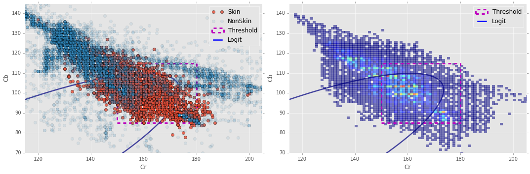

Out [19]:

Notice in the plot on the left I made the non-skin pixels highly transparent; I did this so that the skin pixels would show through better since they are highly entangled with the non-skin pixels.

Clustering skin profiles

Another interesting thing to do is to look at the distribution of skin pixels for individual peoples.

In [20]:

sample_images = ['Srilankan-Actress-Yamuna-Erandathi-001','06Apr03Face','pg42RF','dulani_anuradha4','Matthew_narrowweb__300x381,0']

fig, axes = plt.subplots(len(sample_images),2)
for fn,(ax1,ax2) in zip(sample_images,axes):
    df,img = get_image(fn)
    add_crcb(df)

    ax1.imshow(img)
    ax1.grid(False);ax1.set_xticks([]),ax1.set_yticks([])
    ax1.set_ylabel(fn[:12])
    
    plt.sca(ax2)
    plot_density(df[df.skin == 1],colorbar=False)
    ax2.yaxis.tick_right(); ax2.yaxis.set_label_position("right")
    
axes.item(1).set_title('Skin Pixel Distributions')
fig.set_size_inches(fig.get_size_inches()[0]*1.5, fig.get_size_inches()[0]*2)
fig.tight_layout()
from sklearn.cluster import KMeans

n_clusters=4
km = KMeans(n_clusters=n_clusters,n_init=8,n_jobs=-1)

skin = prath.loc[prath.skin==1,:]
km.fit(skin.loc[:,'Cr':'Cb'])
skin['cluster'] = km.labels_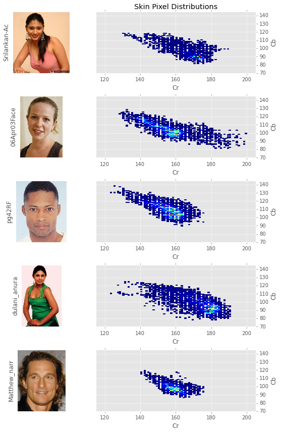

Out [20]:

Although much of the difference in perceived skin color is explained by intensity, chromaticity can also be used as a differentiator among skin profiles. This is most clearly seen when contrasting the South Asian women’s skin profiles - srilankan-Ac and dulani_anura - with the caucasians skin tones. The black man - pg42RF - is somewhat of an anomaly as the highest concentration of skin pixels are in the same region as those of the caucasians.

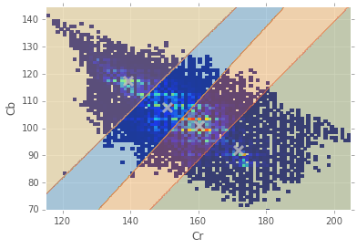
Anyway, we can use a simple K-Means clustering to attempt to get a better idea of how much spread there is in the different skin profiles.

In [21]:

cr = np.linspace(np.min(prath['Cr']),np.max(prath['Cr']),N)
cb = np.linspace(np.min(prath['Cb']),np.max(prath['Cb']),N)

# evaluate the labels over a grid
xx, yy = np.meshgrid(cr,cb)
z = km.predict(np.c_[xx.ravel(), yy.ravel()])

# Put the result into a color plot
z = z.reshape(xx.shape)
plot_density(skin,colorbar=False)
plt.contourf(xx,yy,z,cmap=plt.cm.Paired,alpha=0.4)
centroids = km.cluster_centers_
plt.scatter(centroids[:, 0], centroids[:, 1],
            marker='x', s=100, linewidths=3,
            color='0.75',alpha=0.8)
for i,mean in enumerate(centroids): print "Cluster #{} = {}".format(i,mean)

Out [21]:

Cluster #0 = [ 150.85660996  107.708975  ]
Cluster #1 = [ 171.93326782   91.65710871]
Cluster #2 = [ 160.41745047  100.69489915]
Cluster #3 = [ 139.21217822  117.20015359]

To get a sample of what these clusters actually look like, we randomly sample 180x240 pixels from each cluster to get a “skin palette”. Notice the patches are sorted by their Y component to get a natural gradient and subsequently converted back to RGB in order to show what these skin profiles look like to our natural color perception.

In [22]:

pshape=[180,240]

fig,axes = plt.subplots(1,n_clusters,subplot_kw=dict(xticks=[],yticks=[]))
for i,ax in enumerate(axes):
    plt.sca(ax)
    
    clusterp = skin[skin['cluster'] == i]
    rsamp = np.random.choice(clusterp.index.values,np.product(pshape),replace=False)
    patch = clusterp.ix[rsamp]
    
    patch = patch.sort(columns=['Y']) #sort by luminance value 'Y' for display purposes
    
    imgpatch = patch.loc[:,'r':'b'].values.reshape(pshape+[3]).astype(np.uint8)
    
    ax.imshow(imgpatch,interpolation='nearest')
    ax.grid(False)
    ax.set_title('Skin Cluster #%d' % i)
    
fig.set_size_inches(fig.get_size_inches()[0]*2, fig.get_size_inches()[1]*2)
fig.tight_layout()
fig.subplots_adjust(wspace=0)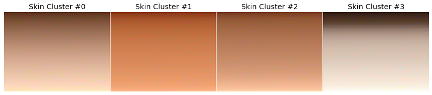

Out [22]:

Let’s see how well these clusters map to each of the different ethnicities in the dataset. For each of our sample images, we’ll show seperately the skin pixels from each cluster.

In [23]:

sample_images = ['Srilankan-Actress-Yamuna-Erandathi-001','06Apr03Face','pg42RF','dulani_anuradha4','Matthew_narrowweb__300x381,0']

fig, axes = plt.subplots(len(sample_images),n_clusters,subplot_kw=dict(xticks=[],yticks=[]))
for fn,subaxes in zip(sample_images,axes):
    imgid,w,h = images.loc[fn]
    
    df = prath.loc[(imgid,),'r':'b']
    skindf = skin.loc[(imgid,),'cluster']
    df = df.join(skindf,how='left') # join skin cluster labels with rgb pixels

    cluster = df.cluster
    df.drop('cluster',inplace=True,axis=1)
    
    for i,ax in enumerate(subaxes):
        img = df.copy()
        img[cluster != i] = 0    
        ax.imshow(img.values.reshape(h,w,3).astype(np.uint8))
        if (i % n_clusters) == 0: ax.set_ylabel(fn[:12])
        
        ax.grid(False)

for i in range(n_clusters):
    axes.item(i).set_title('Skin cluster #%d' % i)

fig.set_size_inches(fig.get_size_inches()[0]*1.5, fig.get_size_inches()[0]*2)
fig.tight_layout()
fig.subplots_adjust(wspace=0,hspace=0)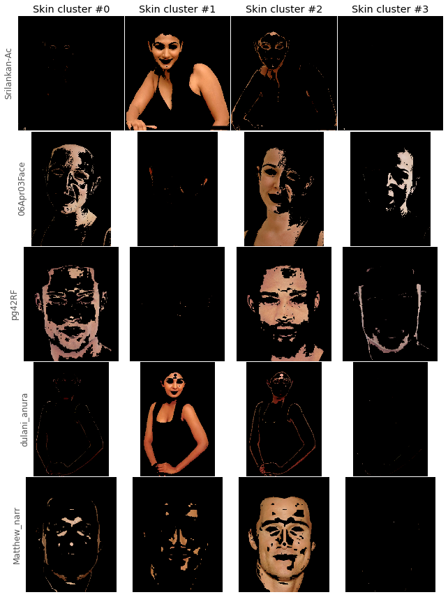

Out [23]:

Just as we speculated above, the South Asian women (cluster #2) are easily distinguishable from the rest of the skin clusters. The caucasians also seem to be modeled well by cluster #3. Cluster #1 is seemingly a garbage cluster, picking up the dim corners of faces. Mr.pg42RF however continues to be difficult to distinguish with a seemingly equal number of skin pixels in two clusters.

Last Notes…

I hope you’ve enjoyed a short look at skin space. I highly encourage any questions or comments you may have. Thanks for reading!

Published: August 01 2015

category: